Jim
Hodges
Extinguished Professor, Division of Biostatistics and Health Data Science, University of Minnesota
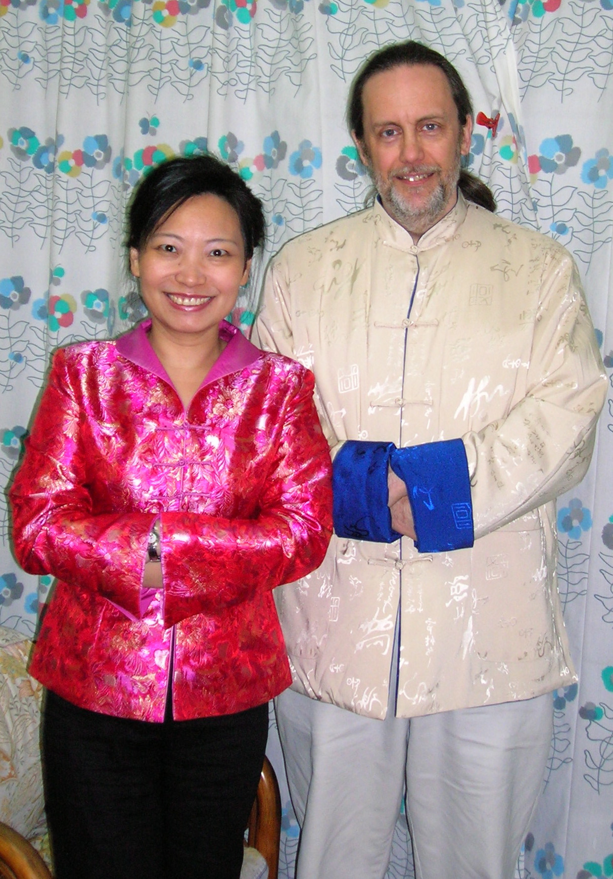
I'm
the one on the right. The one on the left is Li Chi-ping, who became my bride
on 13 February 2007 and inexplicably still is. (Photo taken March 2006, Taipei).
My
location: · Division of Biostatistics and Health Data Science · School of Public Health · University of Minnesota · 2221 University Ave SE, Suite
200 · Minneapolis, Minnesota 55414 · Phone (612) 626-9626, Fax (612)
626-9054 · e-mail:
hodge003@umn.edu, hodges@ccbr.umn.edu (they go to the same inbox) Links · Jim's CV, current as of March 2024 and soporific as ever. · The more-or-less official site
for my book, Richly
Parameterized Linear Models: Additive, Time Series, and Spatial Models Using
Random Effects, which was published by Chapman & Hall in November 2013. · Materials for PubH8492 "Richly Parameterized
Models". The materials are from the Fall 2023 offering of this course. · The supplement for "Statistical methods research done as science rather than mathematics", posted on arXiv at https://arxiv.org/abs/1905.08381. · Some old papers of mine that are hard to find.
Sander Greenland told me I should make them available, so here they are. These
include stat theory papers from the obscure volumes Bayesians produced when
they still saw themselves as a persecuted minority, and some propaganda against
simulation models, especially combat simulation models. · Miscellaneous useful or inspiring things (e.g., a talk on
permutation tests and Feynman on cargo-cult science). Old
links · Regarding the Diversity Visa Lottery 2012. · Manual of Operations, OPT Study, version 1, free
for you to download and crib! Use it at your own risk. · Materials from Summer 2008 VA Methodology Group series:
"Everything is a Mixed Linear Model". · Pre-publication versions of Smoothed ANOVA with application to subgroup analysis,
with authorship varying by version. This was eventually published in Technometrics
in 2007. · Pre-publication versions of "Counting degrees of freedom in hierarchical and other
richly parameterized models", which was eventually published in
Biometrika in 2001. · Items associated with "Some algebra and geometry for hierarchical models,
applied to diagnostics" (JRSSB 1998). I update this page when something changes. Go to the U of M
Biostatistics and Health Data Science home page. Official
Disclaimer: The views and opinions expressed in this page are strictly those of
the page author. The contents of this page have not been approved by the
University of Minnesota. Unofficial
Disclaimer: This is all my fault. Bad statistician! No data!